Another important tool in geospatial data science is the geospatial join. We will introduce the concept with a practical example, and will explain how it is related to the standard join of two tables.
9.1 Motivation
The split-apply-combine pattern that we learned in the previous chapter requires a single geotable with all the relevant information in it. However, many questions in geospatial data science can only be answered with information that is spread across multiple geotables. Hence, the need to join these geotables before attempting to @groupby, @transform and @combine the information.
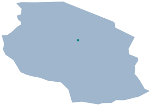
Let’s consider a simple example where we are given two geotables, one containing people who shared their latitude and longitude coordinates:
The georef function has a method that accepts the names of columns with geospatial coordinates. In this example, the table already has the LATITUDE and LONGITUDE coordinates, which we project to a PlateCarree CRS as discussed in the chapter Map projections.
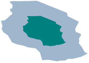
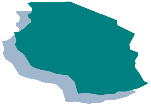
Let’s visualize the geometries of these two geotables:
fig = Mke.Figure()ax = Mke.Axis(fig[1,1], title ="People and countries", xlabel ="Easting [m]", ylabel ="Northing [m]")viz!(countries.geometry)viz!(people.geometry, color ="teal", pointsize =10)fig
Our goal in this example is to attach the “COUNTRY” and “REGION” information to each individual based on their location, represented as a point. In other words, we want to find the countries that contain the location, and then copy the columns to the people.
9.2 Joining geotables
The geojoin function can be used to join two geotables using a geometric predicate function:
geojoin(people, countries, pred =∈)
5×6 GeoTable over 5 PointSet
NAME
AGE
HEIGHT
COUNTRY
REGION
geometry
Categorical
Continuous
Continuous
Categorical
Categorical
Point
[NoUnits]
[yr]
[m]
[NoUnits]
[NoUnits]
🖈 PlateCarree{WGS84Latest}
John
34.0 yr
1.78 m
Brazil
South America
(x: -4.80665e6 m, y: -2.55669e6 m)
Mary
12.0 yr
1.56 m
United States of America
Northern America
(x: -1.35999e7 m, y: 4.16644e6 m)
Paul
23.0 yr
1.7 m
Australia
Australia and New Zealand
(x: 1.70368e7 m, y: -3.05975e6 m)
Anne
39.0 yr
1.8 m
China
Eastern Asia
(x: 1.29584e7 m, y: 4.44205e6 m)
Kate
28.0 yr
1.72 m
missing
missing
(x: -3.60802e6 m, y: -4.28281e5 m)
In the example above, we used the ∈ predicate to check if a Point in the people geotable is in a MultiPolygon in the countries geotable. The default predicate in geojoin is the intersects function that we covered in previous chapters.
Notice that Kate’s “COUNTRY” and “REGION” are missing. That is because Kate lives in the Fernando de Noronha island, which is not present in the countries geotable. To retain just those people for which the geometric predicate evaluates true, we can use a different kind of geojoin known as :inner:
geojoin(people, countries, kind =:inner)
4×6 GeoTable over 4 view(::PointSet, [1, 2, 3, 4])
NAME
AGE
HEIGHT
COUNTRY
REGION
geometry
Categorical
Continuous
Continuous
Categorical
Categorical
Point
[NoUnits]
[yr]
[m]
[NoUnits]
[NoUnits]
🖈 PlateCarree{WGS84Latest}
John
34.0 yr
1.78 m
Brazil
South America
(x: -4.80665e6 m, y: -2.55669e6 m)
Mary
12.0 yr
1.56 m
United States of America
Northern America
(x: -1.35999e7 m, y: 4.16644e6 m)
Paul
23.0 yr
1.7 m
Australia
Australia and New Zealand
(x: 1.70368e7 m, y: -3.05975e6 m)
Anne
39.0 yr
1.8 m
China
Eastern Asia
(x: 1.29584e7 m, y: 4.44205e6 m)
By default, the :left kind is used. Like in standard join, the geojoin is not commutative. If we swap the order of the geotables, the result will be different:
geojoin(countries, people, kind =:inner)
4×6 GeoTable over 4 view(::GeometrySet, [5, 30, 138, 140])
COUNTRY
REGION
NAME
AGE
HEIGHT
geometry
Categorical
Categorical
Categorical
Continuous
Continuous
MultiPolygon
[NoUnits]
[NoUnits]
[NoUnits]
[yr]
[m]
🖈 PlateCarree{WGS84Latest}
United States of America
Northern America
Mary
12.0 yr
1.56 m
Multi(10×PolyArea)
Brazil
South America
John
34.0 yr
1.78 m
Multi(1×PolyArea)
Australia
Australia and New Zealand
Paul
23.0 yr
1.7 m
Multi(2×PolyArea)
China
Eastern Asia
Anne
39.0 yr
1.8 m
Multi(2×PolyArea)
To learn about the different kinds of join, check DataFrames.jl’s documentation on joins.
Note
In database-style join, the predicate function isequal is applied to arbitrary columns of tables. In geojoin, geometric predicate functions are applied to the geometry column of geotables.
The tablejoin function can be used for database-style join between a geotable and a simple table (e.g., DataFrame). The result will be a new geotable over a subset of geometries from the first argument. Please check the documentation for more details.
NoteTip for all users
Besides geojoin, the framework also provides vertical and horizontal concatenation of geotables. Vertical concatenation is achieved with vcat as follows:
All columns are preserved by default, which corresponds to the option kind = :union. Absent columns are filled with missing values. The option kind = :intersect can be used to retain only the columns that are present in all geotables:
vcat(gt1, gt2, kind =:intersect)
6×2 GeoTable over 6 GeometrySet
b
geometry
Categorical
Segment
[NoUnits]
🖈 Cartesian{NoDatum}
4
Segment((x: 0.0 m), (x: 1.0 m))
5
Segment((x: 1.0 m), (x: 2.0 m))
6
Segment((x: 2.0 m), (x: 3.0 m))
4
Segment((x: 0.0 m), (x: 1.0 m))
5
Segment((x: 1.0 m), (x: 2.0 m))
6
Segment((x: 2.0 m), (x: 3.0 m))
Horizontal concatenation is achieved with hcat as follows:
hcat(gt1, gt2)
3×5 GeoTable over 3 CartesianGrid
a
b
b_
c
geometry
Categorical
Categorical
Categorical
Categorical
Segment
[NoUnits]
[NoUnits]
[NoUnits]
[NoUnits]
🖈 Cartesian{NoDatum}
1
4
4
7
Segment((x: 0.0 m), (x: 1.0 m))
2
5
5
8
Segment((x: 1.0 m), (x: 2.0 m))
3
6
6
9
Segment((x: 2.0 m), (x: 3.0 m))
Unique column names are produced with underscore suffixes whenever a column appears in multiple geotables. Julia provides convenient syntax for vcat and hcat:
[gt1
 gt2]
6×4 GeoTable over 6 GeometrySet
a
b
c
geometry
Categorical
Categorical
Categorical
Segment
[NoUnits]
[NoUnits]
[NoUnits]
🖈 Cartesian{NoDatum}
1
4
missing
Segment((x: 0.0 m), (x: 1.0 m))
2
5
missing
Segment((x: 1.0 m), (x: 2.0 m))
3
6
missing
Segment((x: 2.0 m), (x: 3.0 m))
missing
4
7
Segment((x: 0.0 m), (x: 1.0 m))
missing
5
8
Segment((x: 1.0 m), (x: 2.0 m))
missing
6
9
Segment((x: 2.0 m), (x: 3.0 m))
[gt1 gt2]
3×5 GeoTable over 3 CartesianGrid
a
b
b_
c
geometry
Categorical
Categorical
Categorical
Categorical
Segment
[NoUnits]
[NoUnits]
[NoUnits]
[NoUnits]
🖈 Cartesian{NoDatum}
1
4
4
7
Segment((x: 0.0 m), (x: 1.0 m))
2
5
5
8
Segment((x: 1.0 m), (x: 2.0 m))
3
6
6
9
Segment((x: 2.0 m), (x: 3.0 m))
9.3 Common predicates
In geospatial data science, the most common geometric predicates used in geojoin are ∈, ⊆, ==, ≈ and intersects as illustrated in Table 9.1. Specific applications may require custom predicates, which can be easily defined in pure Julia with the Meshes.jl module. For example, it is sometimes convenient to define geometric predicates in terms of a distance and a threshold:
Table 9.1: Common geometric predicates in geospatial join
PREDICATE
EXAMPLE
∈
⊆
==
≈
intersects
9.4 Multiple matches
Sometimes the predicate function will evaluate true for multiple rows of the geotables. In this case, we need to decide which value will be copied to the resulting geotable. The geojoin accepts reduction functions for each column. For example, suppose that Kate decided to move to the continent:
Now, both John and Kate live in Brazil according the countries geotable:
geojoin(people, countries)
5×6 GeoTable over 5 PointSet
NAME
AGE
HEIGHT
COUNTRY
REGION
geometry
Categorical
Continuous
Continuous
Categorical
Categorical
Point
[NoUnits]
[yr]
[m]
[NoUnits]
[NoUnits]
🖈 PlateCarree{WGS84Latest}
John
34.0 yr
1.78 m
Brazil
South America
(x: -4.80665e6 m, y: -2.55669e6 m)
Mary
12.0 yr
1.56 m
United States of America
Northern America
(x: -1.35999e7 m, y: 4.16644e6 m)
Paul
23.0 yr
1.7 m
Australia
Australia and New Zealand
(x: 1.70368e7 m, y: -3.05975e6 m)
Anne
39.0 yr
1.8 m
China
Eastern Asia
(x: 1.29584e7 m, y: 4.44205e6 m)
Kate
28.0 yr
1.72 m
Brazil
South America
(x: -3.97551e6 m, y: -1.07605e6 m)
If we swap the order of the geotables in the geojoin, we need to decide how to reduce the multiple values of “NAME”, “AGE” and “HEIGHT” in the resulting geotable. By default, the mean function is used to reduce Continuous variables, and the first function is used otherwise:
geojoin(countries, people, kind =:inner)
4×6 GeoTable over 4 view(::GeometrySet, [5, 30, 138, 140])
COUNTRY
REGION
NAME
AGE
HEIGHT
geometry
Categorical
Categorical
Categorical
Continuous
Continuous
MultiPolygon
[NoUnits]
[NoUnits]
[NoUnits]
[yr]
[m]
🖈 PlateCarree{WGS84Latest}
United States of America
Northern America
Mary
12.0 yr
1.56 m
Multi(10×PolyArea)
Brazil
South America
John
31.0 yr
1.75 m
Multi(1×PolyArea)
Australia
Australia and New Zealand
Paul
23.0 yr
1.7 m
Multi(2×PolyArea)
China
Eastern Asia
Anne
39.0 yr
1.8 m
Multi(2×PolyArea)
We can specify custom reduction functions using the following syntax:
Congratulations on finishing Part III of the book. Let’s quickly review what we learned so far:
In order to answer geoscientific questions with @groupby, @transform and @combine, we need a single geotable with all the relevant information. This single geotable is often the result of a geojoin with multiple geotables from different sources of information.
There are various kinds of geojoin such as inner and left, which match the behavior of standard join in databases. We recommend the DataFrames.jl documentation to learn more.
The geojoin produces matches with geometric predicate functions. The most common are illustrated in Table 9.1, but custom predicates can be easily defined in pure Julia using functions defined in the Meshes.jl module.
In the next part of the book, you will learn a final important tool that is missing in our toolkit for advanced geospatial data science. The concepts in the following chapters are extremely important.