Overview

Geostatistical functions describe geospatial association of samples based on their locations. These functions have different properties, which are relevant for specific applications, and are documented in the Variograms, Covariances and Transiograms sections.

Below we list the general properties of all geostatistical functions as well as utilities to properly plot, composite and fit these functions to empirical estimates. We illustrate these concepts with variograms given their wide use.

Properties

The following properties can be checked about a geostatistical function:

GeoStatsFunctions.isstationary — Method

isstationary(f)

Check if geostatistical function f possesses the 2nd-order stationary property.

GeoStatsFunctions.isisotropic — Method

isisotropic(f)

Tells whether or not the geostatistical function f is isotropic.

LinearAlgebra.issymmetric — Method

issymmetric(f)

Tell whether or not the geostatistical function f is symmetric.

GeoStatsFunctions.isbanded — Method

isbanded(f)

Tells whether or not the geostatistical function f produces a banded matrix.

GeoStatsFunctions.metricball — Method

metricball(f)

Return the metric ball of the geostatistical function f.

Base.range — Method

range(f)

Return the maximum effective range of the geostatistical function f.

GeoStatsFunctions.nvariables — Method

nvariables(f)

Return the number of (co)variables of the geostatistical function f.

Anisotropy

Anisotropic functions can be constructed from a list of ranges and rotation matrix from Rotations.jl:

γ = GaussianVariogram(ranges = (3.0, 2.0, 1.0), rotation = RotZXZ(0.0, 0.0, 0.0))

GaussianVariogram
├─ ranges: (3.0 m, 2.0 m, 1.0 m)
├─ rotation: [1.0 -0.0 0.0; 0.0 1.0 -0.0; 0.0 0.0 1.0]
├─ sill: 1.0
└─ nugget: 0.0

Rotation angles from commercial geostatistical software are also provided:

GeoStatsBase.MinesightAngles — Type

MinesightAngles(θ₁, θ₂, θ₃)

MineSight z-x'-y'' intrinsic rotation convention following the right-hand rule. All angles are in degrees and the sign convention is CW, CCW, CW positive.

The first rotation θ₁ is a horizontal rotation around the Z-axis, with positive being clockwise. The second rotation θ₂ is a rotation around the new X-axis, which moves the Y-axis into the desired position, with positive direction of rotation is up. The third rotation θ₃ is a rotation around the new Y-axis, which moves the X-axis into the desired position, with positive direction of rotation is up.

References

Sanchez, J. MINESIGHT® TUTORIALS

GeoStatsBase.DatamineAngles — Type

DatamineAngles(θ₁, θ₂, θ₃)

Datamine ZXY rotation convention following the left-hand rule. All angles are in degrees and the signal convention is CW, CW, CW positive. Y is the principal axis.

GeoStatsBase.VulcanAngles — Type

VulcanAngles(θ₁, θ₂, θ₃)

Vulcan ZYX rotation convention following the right-hand rule. All angles are in degrees and the signal convention is CW, CCW, CW positive. X is the principal axis.

GeoStatsBase.GslibAngles — Type

GslibAngles(θ₁, θ₂, θ₃)

GSLIB z-x'-y'' intrinsic rotation convention following the left-hand rule. All angles are in degrees and the sign convention is CW, CCW, CW positive. Y is the principal axis.

The first rotation θ₁ is a rotation around the Z-axis, this is also called the azimuth. The second rotation θ₂ is a rotation around the new X-axis, this is also called the dip. The third rotation θ₃ is a rotation around the new Y-axis, this is also called the tilt.

References

Deutsch, 2015. [The Angle Specification for GSLIB Software] (https://geostatisticslessons.com/lessons/anglespecification)

The effect of anisotropy is clear in the evaluation of the function on any pair of points or geometries:

γ(Point(0, 0, 0), Point(1, 0, 0))

0.2834694059575213

γ(Point(0, 0, 0), Point(0, 1, 0))

0.5276339196255381

γ(Point(0, 0, 0), Point(0, 0, 1))

0.9502129814192044

In the case of isotropic functions, all the results coincide, and one can also use the single argument evaluation with a lag in length units:

γ = GaussianVariogram(range=3.0)

GaussianVariogram
├─ range: 3.0 m
├─ sill: 1.0
└─ nugget: 0.0

γ(1)

0.2834694059575213

Below we illustrate the concept of anisotropy with different rotation angles:

points = rand(Point, 50, crs=Cartesian2D) |> Scale(100)
geotable = georef((Z=rand(50),), points)

viz(geotable.geometry, color = geotable.Z)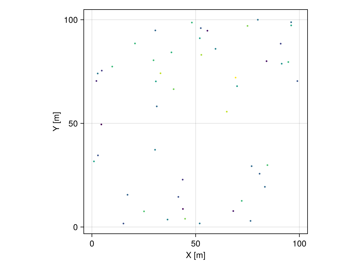

Example block output

θs = range(0.0, step = π/4, stop = 2π - π/4)

# initialize figure
fig = Mke.Figure(size = (800, 1600))

# helper function to position subfigures
pos = i -> CartesianIndices((4, 2))[i].I

# domain of interpolation
grid = CartesianGrid(100, 100)

# anisotropic variogram with different rotation angles
for (i, θ) in enumerate(θs)
  # anisotropic variogram model
  γ = GaussianVariogram(ranges = (20.0, 5.0), rotation = Angle2d(θ))

  # perform interpolation
  interp = geotable |> Interpolate(grid, model=Kriging(γ))

  # visualize solution at subplot i
  viz(fig[pos(i)...],
    interp.geometry, color = interp.Z,
    axis = (title = "θ = $(rad2deg(θ))ᵒ",)
  )
end

fig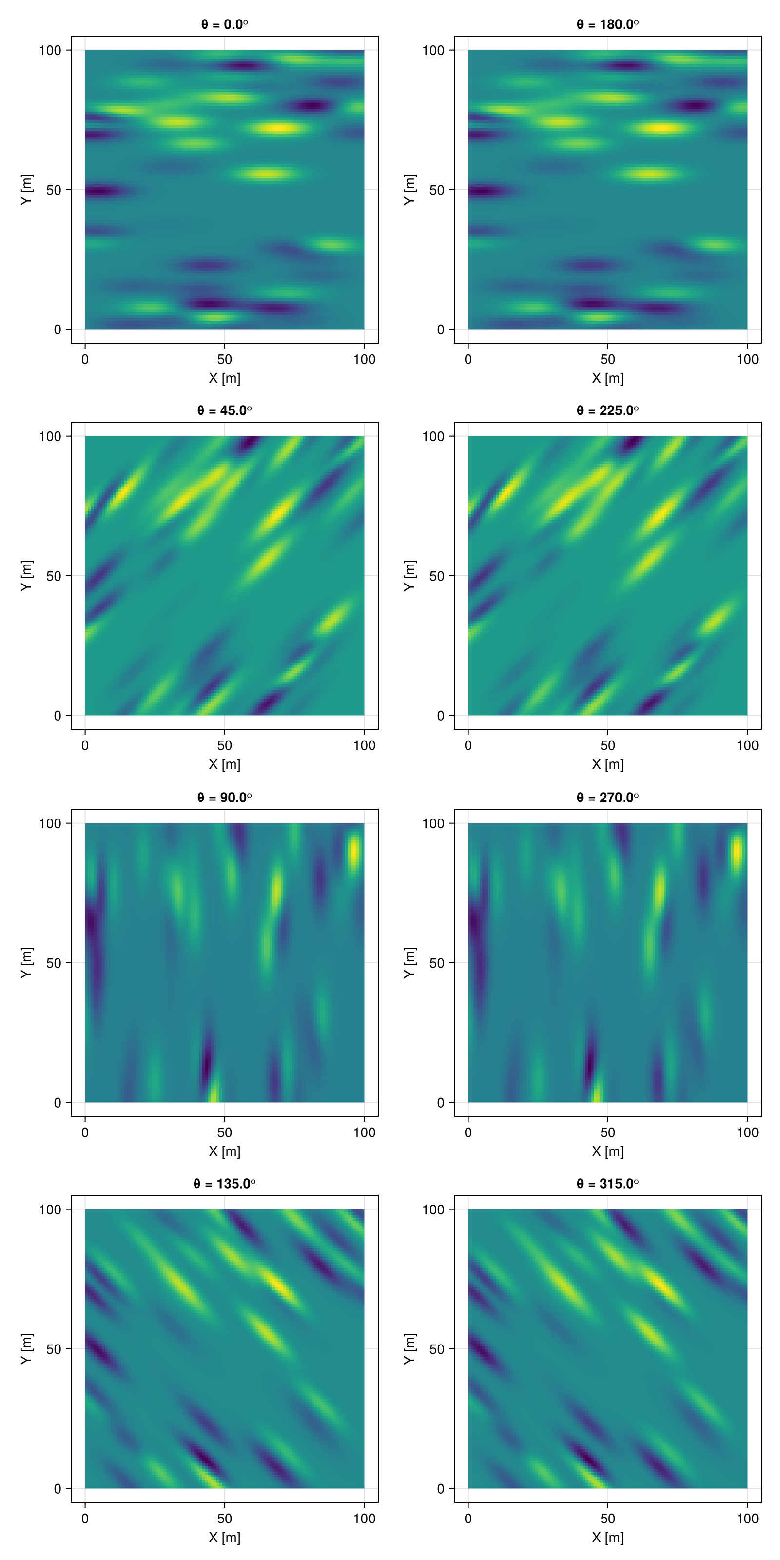

Example block output

Plotting

The function funplot/funplot! can be used to plot any geostatistical function:

GeoStatsFunctions.funplot — Function

funplot(f; [options])

Plot the geostatistical function f with given options.

Common options:

color - color of function graph
linewidth - line width of function graph
maxlag - maximum lag distance

Empirical function options:

linestyle - line style of function graph
pointsize - size of points
showtext - show text counts
textsize - size of text counts
showhist - show histogram
histcolor - color of histogram

Notes

This function will only work in the presence of a Makie.jl backend via package extensions in Julia v1.9 or later versions of the language.

GeoStatsFunctions.funplot! — Function

funplot!(fig, f; [options])

Mutating version of [funplot[@ref] where the figure fig is updated with the plot of the geostatistical function f.

Examples

# initialize figure with Gaussian variogram
fig = funplot(GaussianVariogram())

# add spherical variogram to figure
funplot!(fig, SphericalVariogram())

See the documentation of funplot for options.

Consider the following example with an anisotropic Gaussian variogram:

γ = GaussianVariogram(ranges=(3, 2, 1))

GaussianVariogram
├─ ranges: (3.0 m, 2.0 m, 1.0 m)
├─ rotation: UniformScaling{Bool}(true)
├─ sill: 1.0
└─ nugget: 0.0

funplot(γ)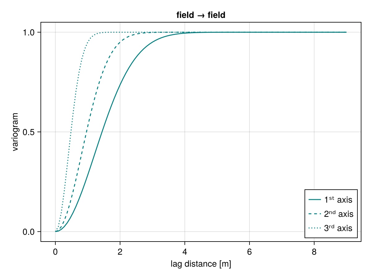

Example block output

The function surfplot/surfplot! can be used to plot surfaces of association given a normal direction:

GeoStatsFunctions.surfplot — Function

surfplot(f; [options])

Plot the geostatistical surface f with given options.

Common options

colormap - Color map
maxlag - maximum lag

Theoretical function options

normal - Normal direction to plane (default to vertical)
nlags - Number of lags (default to 20)
nangs - Number of angles (default to 50)

Examples

# initialize figure with Gaussian variogram
fig = surfplot(GaussianVariogram())

# add spherical variogram to figure
surfplot!(fig, SphericalVariogram())

Notes

This function will only work in the presence of a Makie.jl backend via package extensions in Julia v1.9 or later versions of the language.

GeoStatsFunctions.surfplot! — Function

surfplot!(fig, f; [options])

Mutating version of [surfplot[@ref] where the figure fig is updated with the plot of the geostatistical surface f.

See the documentation of surfplot for options.

surfplot(γ)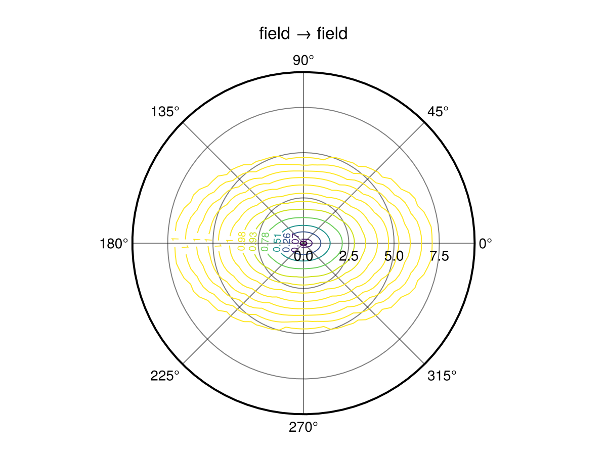

Example block output

Compositing

Composite functions of the form $f(h) = c_1\cdot f_1(h) + c_2\cdot f_2(h) + \cdots + c_n\cdot f_n(h)$ can be constructed using matrix coefficients $c_1, c_2, \ldots, c_n$. The individual structures can be recovered in canonical form with the structures utility:

GeoStatsFunctions.structures — Function

structures(γ)

Return the individual structures of a (possibly composite) variogram as a tuple. The structures are the total nugget, and the coefficients (or contributions) for for the remaining non-trivial structures after normalization (i.e. sill=1, nugget=0).

Examples

γ₁ = GaussianVariogram(nugget=1, sill=2)
γ₂ = SphericalVariogram(nugget=2, sill=3)

structures(2γ₁ + 3γ₂)

structures(cov)

Return the individual structures of a (possibly composite) covariance as a tuple. The structures are the total nugget, and the coefficients (or contributions) for for the remaining non-trivial structures after normalization (i.e. sill=1, nugget=0).

Examples

cov₁ = GaussianCovariance(nugget=1, sill=2)
cov₂ = SphericalCovariance(nugget=2, sill=3)

structures(2cov₁ + 3cov₂)

γ₁ = GaussianVariogram(nugget=1, sill=2)
γ₂ = ExponentialVariogram(nugget=2, sill=3)

# composite model with matrix coefficients
γ = [1.0 0.0; 0.0 1.0] * γ₁ + [2.0 0.5; 0.5 3.0] * γ₂

# structures in canonical form
cₒ, c, g = structures(γ)

cₒ # matrix nugget

2×2 StaticArraysCore.SMatrix{2, 2, Float64, 4} with indices SOneTo(2)×SOneTo(2):
 5.0  1.0
 1.0  7.0

c # matrix coefficients

([1.0 0.0; 0.0 1.0], [2.0 0.5; 0.5 3.0])

g # normalized structures

(GaussianVariogram(range: 1.0 m, sill: 1.0, nugget: 0.0), ExponentialVariogram(range: 1.0 m, sill: 1.0, nugget: 0.0))

funplot(γ) # multivariate funplot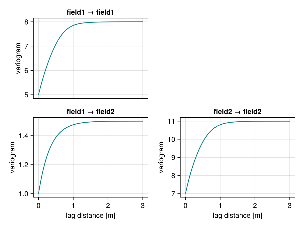

Example block output

surfplot(γ) # multivariate surfplot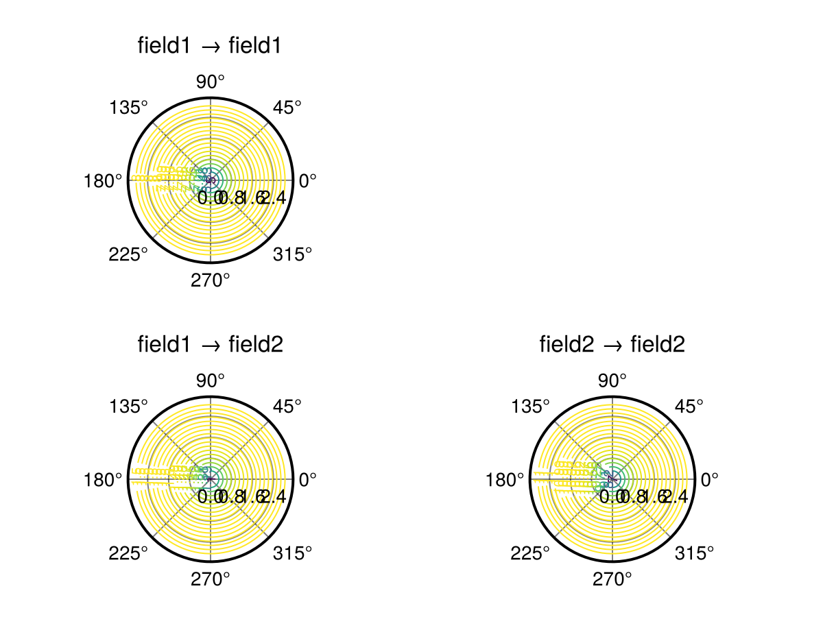

Example block output

Fitting

Fitting theoretical functions to empirical functions is an important modeling step to ensure valid mathematical models of geospatial continuity:

GeoStatsFunctions.fit — Function

fit(F, f, algo=WeightedLeastSquares(); kwargs...)

Fit theoretical geostatistical function of type F to empirical function f using algorithm algo.

Optionally fix theoretical parameters like range, sill and nugget in the kwargs.

Examples

julia> fit(SphericalVariogram, g)
julia> fit(ExponentialVariogram, g)
julia> fit(ExponentialVariogram, g, sill=1.0)
julia> fit(ExponentialVariogram, g, maxsill=1.0)
julia> fit(GaussianVariogram, g, WeightedLeastSquares())

fit(Fs, f, algo=WeightedLeastSquares(); kwargs...)

Fit theoretical geostatistical functions of types Fs to empirical function f using algorithm algo and return the one with minimum error.

Examples

julia> fit([SphericalVariogram, ExponentialVariogram], g)

fit(F, f, weightfun; kwargs...)

Convenience method that forwards the weighting function weightfun to the WeightedLeastSquares algorithm.

Examples

fit(SphericalVariogram, g, h -> exp(-h))
fit(Variogram, g, h -> exp(-h/100))

fit(Variogram, g, algo=WeightedLeastSquares(); kwargs...)

Fit all stationary Variogram models to empirical variogram g using algorithm algo and return the one with minimum error.

Examples

julia> fit(Variogram, g)
julia> fit(Variogram, g, h -> 1 / h)

fit(Transiogram, t, algo=WeightedLeastSquares(); kwargs...)

Fit all theoretical Transiogram models to empirical transiogram t using algorithm algo and return the one with minimum error.

Examples

julia> fit(Transiogram, t)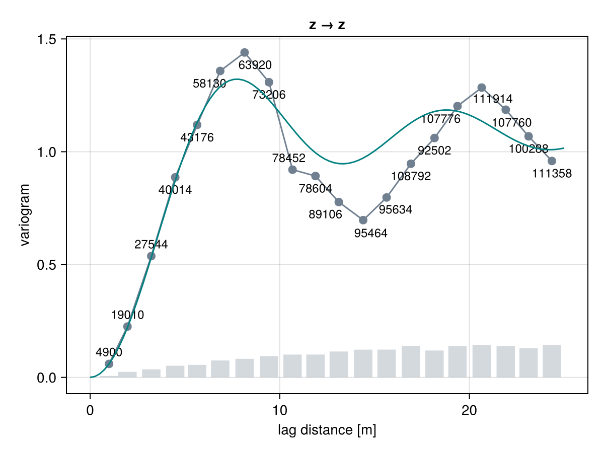
julia> fit(Transiogram, t, h -> 1 / h)

Consider the following EmpiricalVariogram as an example:

# sinusoidal data
data = georef((z=[sin(i/2) + sin(j/2) for i in 1:50, j in 1:50],))

# empirical variogram
g = EmpiricalVariogram(data, "z", maxlag = 25u"m")

funplot(g)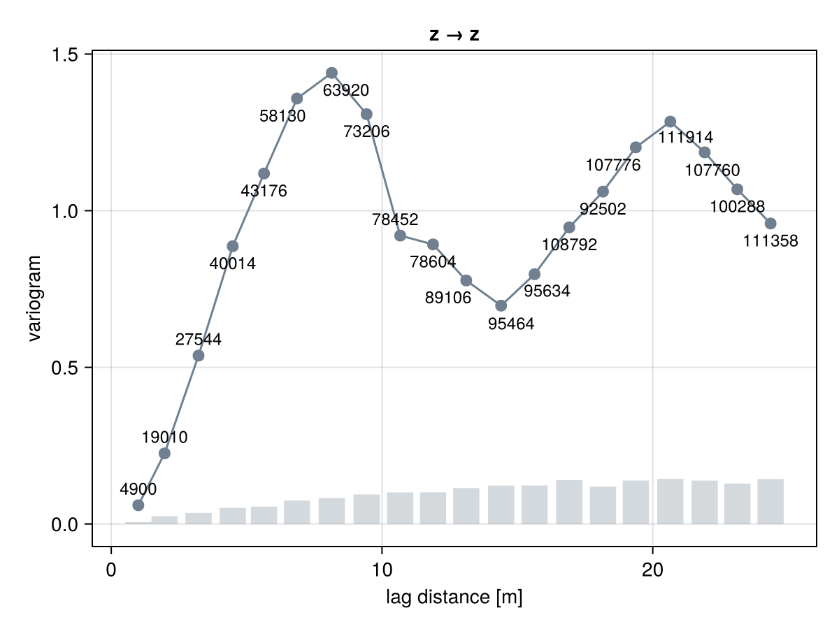

Example block output

We can fit a specific theoretical variogram such as the SineHoleVariogram with

γ = GeoStatsFunctions.fit(SineHoleVariogram, g)

fig = funplot(g)
funplot!(fig, γ, maxlag = 25u"m")

Example block output

or we can let the framework find the theoretical variogram with minimum error:

γ = GeoStatsFunctions.fit(Variogram, g)

fig = funplot(g)
funplot!(fig, γ, maxlag = 25u"m")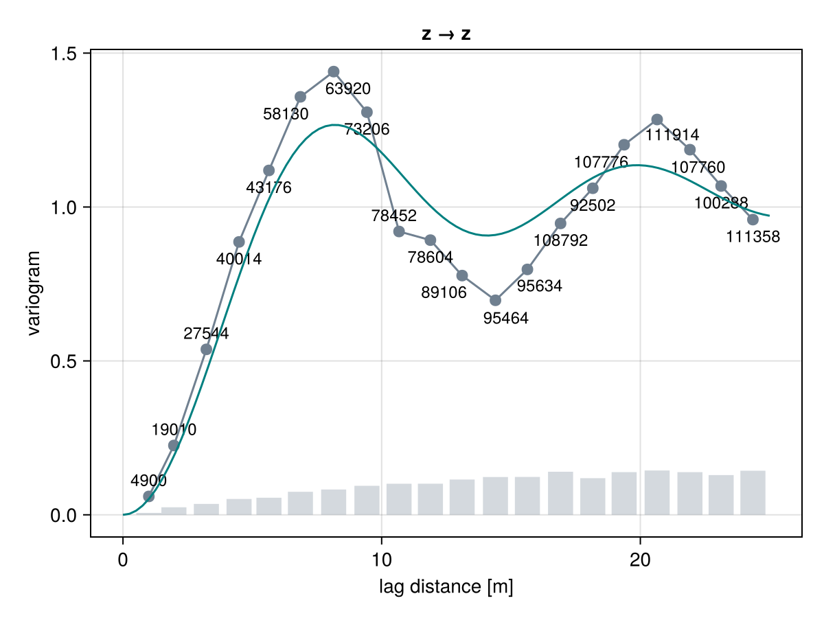

Example block output

The SineHoleVariogram fits the empirical variogram well given that this is a sinusoidal field.

We can also provide a list of candidate models and let framework decide which one has the best fit:

γ = GeoStatsFunctions.fit([GaussianVariogram, SphericalVariogram], g)

fig = funplot(g)
funplot!(fig, γ, maxlag = 25u"m")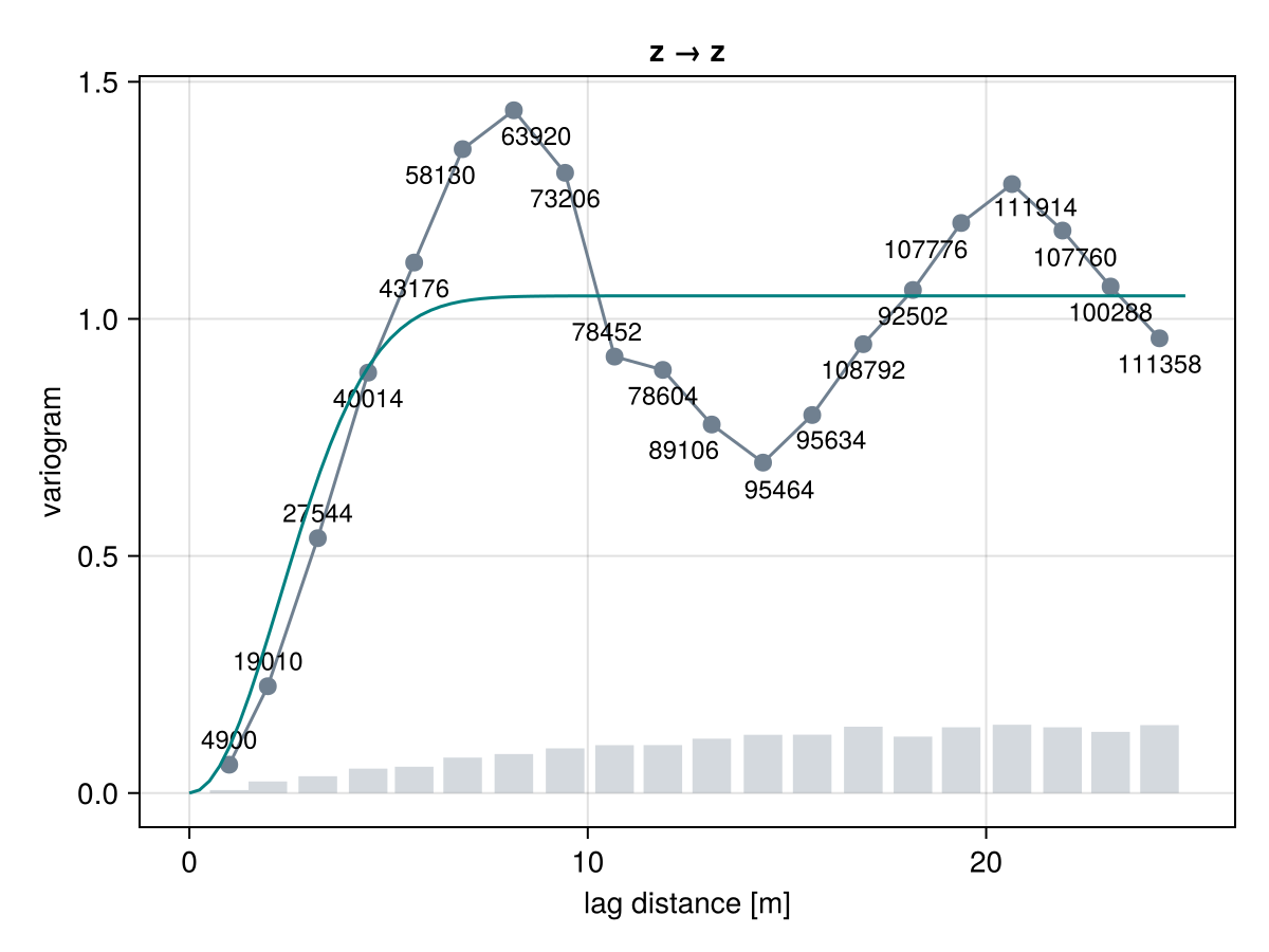

Example block output

Finally, we can fix specific parameters during the optimization by passing them as keyword arguments:

γ = GeoStatsFunctions.fit(SineHoleVariogram, g, sill=1.2)

fig = funplot(g)
funplot!(fig, γ, maxlag = 25u"m")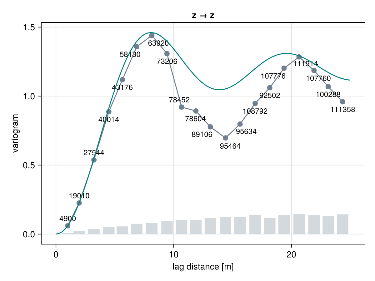

Example block output

and can specify a custom weight function w(h) that informs how important is the misfit at any given lag h:

γ = GeoStatsFunctions.fit(SineHoleVariogram, g, h -> 1 / h^2)

fig = funplot(g)
funplot!(fig, γ, maxlag = 25u"m")

Example block output